
Manipulating Imported .CSV Data Files in Excel
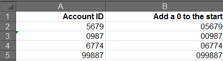
Manipulating Imported CSV Data Files in Excel. Let’s look at a scenario where data is given to you in .CSV format or already has been imported into Excel for you. It may be the case that you have a list of ID numbers, when they are pasted or imported into Excel, the leading Zero which was there in the database that you took them from disappears when it arrives in Excel, as Excel deletes a zero at the front of all numbers. See example below:
| Account ID |
| 5679 |
| 0987 |
| 6774 |
| 99887 |
In order for this list to be valid, you need to insert a 0 (zero) infront of each of the ID numbers. To do this we can use the formula CONCATENATE or the “&” operator.
Using the COCATENTATE formula:
CONCATENATE joins together the values, or cell values to show in one cell. Take for example the following:
We need to take the contents of the cells in Column A and then add a zero to the start of each one. The formula would be as follows:
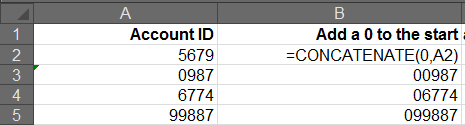
This takes the 0 and then joins it to the front of the contents of cell A2.
As you can see from above Column B now shows a leading zero in front of each of the ids.
Using the “&” Operator:
The “&” symbol can also be used to get the same answer. Most of the time, we find ourselves using the “&” symbol instead of concatenate as it is actually easier!
This time the formula to join the 0 and the cell value would look like this:
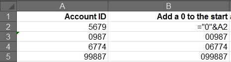
We are literally taking the “0” and joining it to the value of the cell A2.
Great you might say – but wait…. as you can see, some of the numbers already had a leading zero, now they have two zeros and that is not what we wanted! So what we can do is put this formula into an IF statement.
Using an IF statement
In order for us to find if the zero is there already, we are going to use the formula =LEFT(). This will allow is to check to see if the first left most character in the cell is equal to zero.
Here is the finished formula, let’s see how we built it:
=IF(LEFT(A2,1)=”0″, A2, “0”&A2)
Let’s break it down into sections to explain it:
=LEFT(A2,1)
This means, start at the left of cell A2 and go in one character
=LEFT(A2,1)=”0″
This means find the first charcter of cell A2 and see if it equal to zero. Why is the zero in quotes (“0”)? Because in Excel it is most likely being stored as text, so we need to treat it like text and to do so means to put it into quotes.
Now the IF statement:
Condition to check: =LEFT(A2,1)=”0″
If the condition above is True, then no need to add a zero, so leave the value as it is already in A2
If the condition above is False, the we need to join a “0” to A2 by using the & symbol “0”&A2
So, complete formula is:
=IF(LEFT(A2,1)=”0″,
A2, “0”&A2)
Give it a Go!!
Be Brilliant at Excel. Save Hours each week and add Professional Certification to Your Resume
Even Microsoft use us to teach their employees Excel
Get access to The Ultimate Excel Training Course Bundle